Excel VBA: Color Banding AKA Highlight Alternating Rows

Building on the previous posts getLastRow() and getLastCol(), here is an example application of those techniques.

There are many ways to have alternating background color on rows in Excel: there’s a built-in option if you are working with a table, you can use conditional formatting with a formula, or add a helper column to filter and highlight manually. I find that having the color alternate on every single row doesn’t always suit the data I am working with however – often I would rather have the color change help me identify changes in one or more columns that are sorted so I can notice where one chunk ends and another begins.

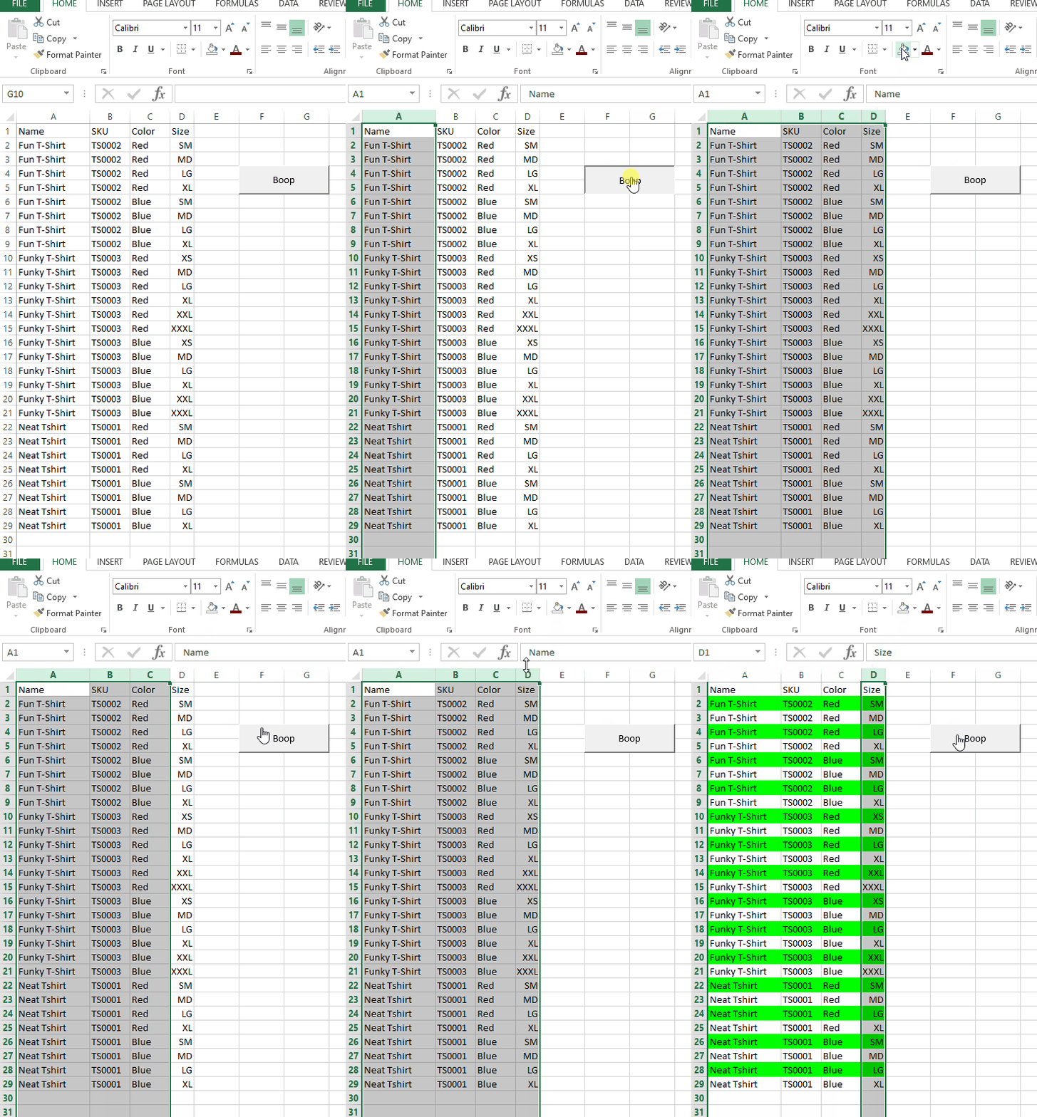
This macro considers the content of the column(s) that are selected and alternates the background color each time it changes. This is probably easier to understand in a picture, so here we go:

The concept is simple: starting from the top, every time the contents of the selected column differ from the row above, that group of cells will either be highlighted or left alone. I designed this so that multiple columns could be selected – in the animation above you can see at first when only column A is selected that there are three highlighted groups, but when A:C is selected that there are six groups of rows.

If only a range of cells are selected rather than an entire column, the highlighting will be confined to those rows. When the entire column is selected it will only extend to the last used row and ignore the blanks at the bottom of the sheet – this is where the getLastRow() function comes into play. Additionally, the highlighted area stretches from column A to the last used column – found with the getLastCol() function.

The Code

Sub colorBands()

'highlight a range that contains the changing values to higlight by
'the range from column A to the last column will be alternatingly highlighted
'not intended for non-continuous selections

Dim s As Worksheet
Set s = ActiveSheet

Dim startRowNum As Long
Dim endRowNum As Long 'if the whole column is selected, only higlight to the last used row
Dim startColNum As Long
Dim endColNum As Long
Dim prevValue As Variant
Dim values As Variant 'the whole set will be added to an array for comparison
Dim startRows As Variant 'each set of rows will have a start and end in an array
Dim endRows As Variant
Dim rowOffset As Long 'difference between the row number and the counter variables
Dim colOffset As Long
Dim rowCount As Long
Dim colCount As Long
Dim lastCol As Long
Dim i As Long
Dim j As Long
Dim k As Long
Dim m As Long 'skip L because it's hard to differentiate from i
Dim n As Long
Dim tempValue As Variant
Dim highlight As Boolean

ReDim values(1 To 1)

'find the boundaries of the selection
endColNum = getLastCol()
endRowNum = getLastRow()
startColNum = Selection.Column
startRowNum = Selection.row
endColNum = startColNum + Selection.Columns.Count - 1
If startRowNum + Selection.Rows.Count < endRowNum Then endRowNum = startRowNum + Selection.Rows.Count - 1 'reset the row limit to highlight if the selection doesn't reach the end of the data in that column
rowOffset = startRowNum - 1
colOffset = startColNum - 1
rowCount = endRowNum - startRowNum + 1
colCount = endColNum - startColNum + 1
lastCol = getLastCol(, startRowNum)

'Some output for troubleshooting
Debug.Print "Starting Column: " & startColNum
Debug.Print "Ending Column: " & endColNum
Debug.Print "Starting Row: " & startRowNum
Debug.Print "Ending Row: " & endRowNum
Debug.Print "Offset from row 1 by: " & rowOffset
Debug.Print "Row Count: " & rowCount
Debug.Print "Column Count: " & colCount

'add the values to an array
If startColNum = endColNum Then
    For i = 1 To rowCount
        ReDim Preserve values(1 To i)
        values(i) = s.Cells(i + rowOffset, startColNum).Value
    Next i
Else
    For i = 1 To rowCount
        ReDim Preserve values(1 To i)
        For j = 1 To colCount
            tempValue = tempValue & s.Cells(i + rowOffset, j + colOffset).Value
        Next j
        values(i) = tempValue
        tempValue = Empty
    Next i
End If

'define the ranges that need to be higlighted
ReDim startRows(1 To 1)
ReDim endRows(1 To 1)
startRows(1) = startRowNum

m = 1
highlight = False
For k = 2 To rowCount
    If values(k) <> values(k - 1) Then 'this row is different from the previous, so it should start or end a higlighted area
        If highlight = False Then 'start a highlighted area
            ReDim Preserve startRows(1 To m)
            ReDim Preserve endRows(1 To m)
            highlight = True
            startRows(m) = k
        Else                    'end a highlighted area
            highlight = False
            endRows(m) = k - 1
            m = m + 1
        End If
    End If
Next k

If highlight = True Then endRows(m) = endRowNum - rowOffset 'close the last range if it's dangling

'Highlight each block
For n = 1 To UBound(startRows)
    s.Range(s.Cells(startRows(n) + rowOffset, 1), s.Cells(endRows(n) + rowOffset, lastCol)).Interior.ColorIndex = 4 'change this for a different color
Next n

End Sub

How to use it

In order to use this, I recommend adding it to your personal.xlsb file and mapping it to a button in the toolbar or a keyboard shortcut. The two functions getLastRow() and getLastCol() are also required, so those will also have to be added to the file. As I write more of these shared functions I will keep a single file up to date here to make this installation easier (link directly below).

Tips

• Save frequently, particularly before executing a macro. You cannot undo a macro, if something goes wrong you could lose work.
• Clear existing background colors before using this
• Change the color to something other than green if you prefer
• Avoid using this while filtered or with discontinuous selections, or you may get unexpected results
• This isn’t optimized for performance in any way, so be wary when using it on something large for the first time. For 50k rows it took ~5 seconds on my machine.