Tag: Excel

Here are two functions that I will be using in an upcoming sheet, I want to explain them briefly and add them to my small library (file is downloadable at the end of this post).

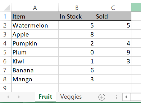
The names hint at the purpose: given a value to match, they will return the number of the row or column the value was found in, or zero if it wasn’t found at all. The concept is similar to the “vlookup” formula, but performance for these two functions is terrible by comparison and for that reason I don’t recommend using them repetitively in a loop or with large columns of data. I maintain several files with built-in functionality where most of the user input comes from cells in a sheet but I can’t always guarantee the position of those cells – that’s where these two come in handy. Instead of hard-coding the cell address, these functions can find the address by matching the value in that cell which allows you to modify the user-facing sheet without having to update code every time; it also makes the sheet somewhat tolerant of being rearranged by the user, but you need to be careful in case it’s been mangled in such a way that the inputs are found but are totally bogus.

getRowNum()

Function getRowNum(findValue As Variant, Optional sheetName As String, Optional colNum As Long) As Long
'by Elliot 8/9/20 www.elliotmade.com
'this function will return the row number in the first (or specified) column that matches the "findValue" parameter
'this is similar to vlookup, but not as fast or performant
'an example use is to get an input from a sheet where you can't guarantee the position of the cell
'combine this with getColNum() to find a cell value where a known column heading and row label intersect
'****** this requires the "getlastrow" function *******

Dim i As Long
Dim lastRow As Long

Dim j As Long
If sheetName <> "" Then
    For j = 1 To Worksheets.Count
        If Worksheets(j).Name = sheetName Then GoTo sheetOK
    Next j
    GoTo abort 'specified sheet name was not found
sheetOK:
End If

'default values for optional parameters
If sheetName = "" Then sheetName = ActiveSheet.Name
If colNum = 0 Then colNum = 1

lastRow = getLastRow(sheetName, colNum)

For i = 1 To lastRow
    If Worksheets(sheetName).Cells(i, colNum).Value2 = findValue Then
        getRowNum = i
        GoTo found
    End If
Next i

found:
abort:

End Function

getColNum()

Function getColNum(findValue As Variant, Optional sheetName As String, Optional rowNum As Long) As Long
'by Elliot 8/9/20 www.elliotmade.com
'this function will return the column number in the first (or specified) column that matches the "findValue" parameter
'this is similar to vlookup, but inverted not as fast or performant
'an example use is to get an input from a sheet where you can't guarantee the position of the cell
'combine this with getRowNum() to find a cell value where a known column heading and row label intersect
'****** this requires the "getLastCol" function *******

Dim i As Long
Dim lastCol As Long

Dim j As Long
If sheetName <> "" Then
    For j = 1 To Worksheets.Count
        If Worksheets(j).Name = sheetName Then GoTo sheetOK
    Next j
    GoTo abort 'specified sheet name was not found
sheetOK:
End If

'default values for optional parameters
If sheetName = "" Then sheetName = ActiveSheet.Name
If rowNum = 0 Then rowNum = 1

lastCol = getLastCol(sheetName, rowNum)

For i = 1 To lastCol
    If Worksheets(sheetName).Cells(rowNum, i).Value2 = findValue Then
        getColNum = i
        GoTo found
    End If
Next i

found:
abort:

End Function

The usage for both of these is simple, just give them a value to match, and if you want to search in a different row/column or a different sheet use the optional parameters. Note that these both rely on two functions I posted previously – getLastRow() and getLastCol(), both of which are included in the file below as well.

Building on the previous posts getLastRow() and getLastCol(), here is an example application of those techniques.

There are many ways to have alternating background color on rows in Excel: there’s a built-in option if you are working with a table, you can use conditional formatting with a formula, or add a helper column to filter and highlight manually. I find that having the color alternate on every single row doesn’t always suit the data I am working with however – often I would rather have the color change help me identify changes in one or more columns that are sorted so I can notice where one chunk ends and another begins.

This macro considers the content of the column(s) that are selected and alternates the background color each time it changes. This is probably easier to understand in a picture, so here we go:

The concept is simple: starting from the top, every time the contents of the selected column differ from the row above, that group of cells will either be highlighted or left alone. I designed this so that multiple columns could be selected – in the animation above you can see at first when only column A is selected that there are three highlighted groups, but when A:C is selected that there are six groups of rows.

If only a range of cells are selected rather than an entire column, the highlighting will be confined to those rows. When the entire column is selected it will only extend to the last used row and ignore the blanks at the bottom of the sheet – this is where the getLastRow() function comes into play. Additionally, the highlighted area stretches from column A to the last used column – found with the getLastCol() function.

The Code

Sub colorBands()

'highlight a range that contains the changing values to higlight by
'the range from column A to the last column will be alternatingly highlighted
'not intended for non-continuous selections

Dim s As Worksheet
Set s = ActiveSheet

Dim startRowNum As Long
Dim endRowNum As Long 'if the whole column is selected, only higlight to the last used row
Dim startColNum As Long
Dim endColNum As Long
Dim prevValue As Variant
Dim values As Variant 'the whole set will be added to an array for comparison
Dim startRows As Variant 'each set of rows will have a start and end in an array
Dim endRows As Variant
Dim rowOffset As Long 'difference between the row number and the counter variables
Dim colOffset As Long
Dim rowCount As Long
Dim colCount As Long
Dim lastCol As Long
Dim i As Long
Dim j As Long
Dim k As Long
Dim m As Long 'skip L because it's hard to differentiate from i
Dim n As Long
Dim tempValue As Variant
Dim highlight As Boolean

ReDim values(1 To 1)

'find the boundaries of the selection
endColNum = getLastCol()
endRowNum = getLastRow()
startColNum = Selection.Column
startRowNum = Selection.row
endColNum = startColNum + Selection.Columns.Count - 1
If startRowNum + Selection.Rows.Count < endRowNum Then endRowNum = startRowNum + Selection.Rows.Count - 1 'reset the row limit to highlight if the selection doesn't reach the end of the data in that column
rowOffset = startRowNum - 1
colOffset = startColNum - 1
rowCount = endRowNum - startRowNum + 1
colCount = endColNum - startColNum + 1
lastCol = getLastCol(, startRowNum)

'Some output for troubleshooting
Debug.Print "Starting Column: " & startColNum
Debug.Print "Ending Column: " & endColNum
Debug.Print "Starting Row: " & startRowNum
Debug.Print "Ending Row: " & endRowNum
Debug.Print "Offset from row 1 by: " & rowOffset
Debug.Print "Row Count: " & rowCount
Debug.Print "Column Count: " & colCount

'add the values to an array
If startColNum = endColNum Then
    For i = 1 To rowCount
        ReDim Preserve values(1 To i)
        values(i) = s.Cells(i + rowOffset, startColNum).Value
    Next i
Else
    For i = 1 To rowCount
        ReDim Preserve values(1 To i)
        For j = 1 To colCount
            tempValue = tempValue & s.Cells(i + rowOffset, j + colOffset).Value
        Next j
        values(i) = tempValue
        tempValue = Empty
    Next i
End If

'define the ranges that need to be higlighted
ReDim startRows(1 To 1)
ReDim endRows(1 To 1)
startRows(1) = startRowNum

m = 1
highlight = False
For k = 2 To rowCount
    If values(k) <> values(k - 1) Then 'this row is different from the previous, so it should start or end a higlighted area
        If highlight = False Then 'start a highlighted area
            ReDim Preserve startRows(1 To m)
            ReDim Preserve endRows(1 To m)
            highlight = True
            startRows(m) = k
        Else                    'end a highlighted area
            highlight = False
            endRows(m) = k - 1
            m = m + 1
        End If
    End If
Next k

If highlight = True Then endRows(m) = endRowNum - rowOffset 'close the last range if it's dangling

'Highlight each block
For n = 1 To UBound(startRows)
    s.Range(s.Cells(startRows(n) + rowOffset, 1), s.Cells(endRows(n) + rowOffset, lastCol)).Interior.ColorIndex = 4 'change this for a different color
Next n

End Sub

How to use it

In order to use this, I recommend adding it to your personal.xlsb file and mapping it to a button in the toolbar or a keyboard shortcut. The two functions getLastRow() and getLastCol() are also required, so those will also have to be added to the file. As I write more of these shared functions I will keep a single file up to date here to make this installation easier (link directly below).

Tips

• Save frequently, particularly before executing a macro. You cannot undo a macro, if something goes wrong you could lose work.
• Clear existing background colors before using this
• Change the color to something other than green if you prefer
• Avoid using this while filtered or with discontinuous selections, or you may get unexpected results
• This isn’t optimized for performance in any way, so be wary when using it on something large for the first time. For 50k rows it took ~5 seconds on my machine.

Similar to my previous post on finding the last used row in a sheet, this is a function that can be used to find the last used column. These two functions work nicely together to limit a loop or define a range when the source data may vary in size.

The function: getLastCol():

• If called with no parameters, the last used column in the active worksheet will be returned.
• The optional sheetName parameter lets you reference a sheet other than the one that is active.
• The optional rowNum parameter returns the last used column in a particular row.
• The optional colLimit parameter limits the total number of iterations in the loop when searching for the last used column, this can be used to speed up execution when you have an idea of what the sheet may contain already.
• If there is an error with the parameters it will return zero

Examples:

getLastCol() = 3
getLastCol("Fruit") = 3
getLastCol(,3) = 2 'last used column on row 3 only
getLastCol(Vegetables) = 0 'this sheet name does not exist

The Code:

Function getLastCol(Optional sheetName As String, Optional rowNum As Long, Optional colLimit As Long) As Long
'by Elliot 7/22/20 www.elliotmade.com
'this function will return the last used column on a sheet in a single row
'if no sheet name is specified it will use the active sheet
'if no row is specified it will find the last column in any row up to an optional limit (for faster performance)
'two assumptions are made: the file type is .xlsx or similar that supports 16k columns
'and the sheet is in the active workbook
'a zero returned means that there was a failure

Dim i As Long
Dim j As Long
Dim curLastCol As Long

'check for valid inputs first, return zero if there is a problem
If rowNum < 0 Or rowNum > 1048575 Then GoTo abort

If sheetName <> "" Then
    For i = 1 To Worksheets.Count
        If Worksheets(i).Name = sheetName Then GoTo sheetOK
    Next i
    GoTo abort 'specified sheet name was not found
sheetOK:
End If

If colLimit = 0 Then
    colLimit = 16384
ElseIf colLimit < 0 Or colLimit > 16384 Then
    GoTo abort
End If

If sheetName = "" Then sheetName = ActiveSheet.Name

'if no problem, find the last column
If rowNum = 0 Then
    getLastCol = Worksheets(sheetName).Cells(1, 16384).End(xlToLeft).Column
    For j = 1 To colLimit
        If Worksheets(sheetName).Cells(1048575, j).End(xlUp).Row > 1 Then curLastCol = j
        If curLastCol > getLastCol Then getLastCol = curLastCol
    Next j
Else
    getLastCol = Worksheets(sheetName).Cells(rowNum, 16384).End(xlToLeft).Column
End If

abort:

End Function

You may notice that the method using xlToLeft is used to find the last column in a specific row, but I did not use it when searching for the last column in the entire sheet; to do this in a loop would require iterating through every single row (over 1M!) and would take a significant amount of time. I chose to do two things to shortcut this process: first, check the first row because it often has headings for the rest of the document, and second, find the last used row in every column instead. This limits the possible trips through the loop to 16k at most (the number of columns in a sheet). I have some other ideas to improve on this, but I’ll leave it alone for now until it becomes a bottleneck.

Next I’ll post an example that puts this function to use, stay tuned.

If you’re getting into Excel macros and have fooled around with the macro recorder you may notice that the resulting code is very rigid: it only works on the exact range of cells you had selected for example (among other drawbacks). In many cases you want your code to adapt to the size of the data in a sheet, and for this you need to determine the boundaries of the range.

.UsedRange Property

If you’ve done a search you may have come across this approach already. .UsedRange.Rows.Count will usually give the right result if you’re looking for the last used row on a particular sheet, but not always. For whatever reason, this property is not always current – sometimes it is possible to clear the contents of a row without causing this to update, giving an incorrect result. Saving the document (and probably some other actions) will cause this to be updated, but I don’t consider it to be reliable enough to base further logic on.

.End(xlUp).row

This approach is the equivalent of putting your cursor in a cell and pushing CTRL+UP. If you do this on the very last row of a sheet, the cell that your cursor lands on will be the last one in that column. This works reliably, but only gives a result for one column, not the entire sheet. If you put this together with a loop and repeat it for all columns (or a reasonable number) you can reliably retrieve the last used row on a sheet.

The function: getLastRow()

Putting this all together, an easy to use function can be made that returns the last row number on a sheet or in a specific column.

• If called with no parameters it will return the last used row in the first 100 columns of the active sheet.
• The optional sheetName parameter is useful to reference a sheet other than the active one, or if you can’t guarantee which sheet is active when the function is called.
• The second optional parameter, colNum, can be used if you want to know the last used row in a specific column.

Examples

Here are some examples of how this works with the sample sheet below:

getLastRow() = 8 'from the active sheet
getLastRow("Fruit") = 8 'even when a different sheet is active
getLastRow(,3) = 6 'from the active sheet
getLastRow("Fruit", 3) = 6 'even when a different sheet is active
getLastRow("Fruit", 4) = 1 'this column is empty
getLastROW("Vegetables") = 0 'this sheet name is invalid

And finally, the function itself:

Function getLastRow(Optional sheetName As String, Optional colNum As Long) As Long
'by Elliot 7/22/20 www.elliotmade.com
'this function will return the last used row on a sheet or a single row
'if no sheet name is specified it will use the active sheet
'if no column is specified it will find the last row in any of the first 100 columns
'two assumptions are made: the file type is .xlsx or similar that supports ~1M rows
'and the sheet is in the active workbook

'a zero returned means that there was a failure

Dim i As Long
Dim j As Long
Dim curLastRow As Long

'check for valid inputs first, return zero if there is a problem
If colNum < 0 Or colNum > 16384 Then GoTo abort

If sheetName <> "" Then
    For j = 1 To Worksheets.Count
        If Worksheets(j).Name = sheetName Then GoTo sheetOK
    Next j
    GoTo abort 'specified sheet name was not found
sheetOK:
End If

If sheetName = "" Then sheetName = ActiveSheet.Name

'if no problem, find the last row
If colNum = 0 Then
For i = 1 To 100
    curLastRow = Worksheets(sheetName).Cells(1048575, i).End(xlUp).Row
    If curLastRow > getLastRow Then getLastRow = curLastRow
Next i

Else
    curLastRow = Worksheets(sheetName).Cells(1048575, colNum).End(xlUp).Row
End If

abort:

getLastRow = curLastRow

End Function

If you found this useful, or if you have a problem this might help you solve, let me know!

I saw this: https://hackaday.com/2020/04/13/john-horton-conway-creator-of-conways-game-of-life-has-died/, decided that I would try to write his game myself. This was just for fun and it isn’t optimized for anything really, but it might be useful to check out if you are getting into macros for Excel and need to read/update cells in a worksheet.

If you’re not comfortable downloading an .xlsm from (which is wise), the code below can just be pasted in an empty module. Make sure to name a sheet in your workbook “Life”, type in a number in cell B9 (or hardcode it), and add buttons to call the subs if you want.

The black cells are 1’s, white cells are 0’s. Might be interesting to tweak this so it generates QR codes and see where it takes you!

Option Explicit

'by Elliot (elliotmade.com) 4/14/2020
'Conway's game of life

'there is no input validation, and literally no optimization for anything
'wrote this purposely without looking at any examples other than a description of the rules, just for fun

'rules (from wikipedia):
'    Any live cell with two or three live neighbors survives.
'    Any dead cell with three live neighbors becomes a live cell.
'    All other live cells die in the next generation. Similarly, all other dead cells stay dead.

Dim xMax As Long
Dim yMax As Long

Dim x As Long
Dim y As Long

Dim xOffset As Long 'so it doesn't have to occupy the top and left cells
Dim yOffset As Long

Dim ws As Worksheet
Dim ticks As Long
Dim maxTicks As Long

Dim currentGrid() As Byte
Dim nextGrid() As Byte


Sub initialize()
'read in the initial state

xMax = 40
yMax = 40
ticks = 0

xOffset = 3
yOffset = 3

Set ws = Worksheets("Life")

ReDim currentGrid(1 To xMax, 1 To yMax)
ReDim nextGrid(1 To xMax, 1 To yMax)

For y = 1 To yMax
    
    For x = 1 To xMax
        currentGrid(x, y) = ws.Cells(y + yOffset, x + xOffset)
    Next x
Next y

maxTicks = ws.Cells(9, 2).Value


Debug.Print "Initialized"

End Sub

Sub clear()
    Call initialize
    ws.Range(ws.Cells(1 + yOffset, 1 + xOffset), ws.Cells(yMax + yOffset, xMax + xOffset)).Value = 0
    Call initialize
    Call output
    Debug.Print "Cleared"

End Sub

Sub tick()
'really should do initialize if the variables aren't populated...

Dim countNeighbors As Integer

For y = 1 To yMax
    For x = 1 To xMax
        countNeighbors = 0
        'top neighbor
        If y > 1 Then
            countNeighbors = countNeighbors + currentGrid(x, y - 1)
        End If
        'bottom neighbor
        If y < yMax Then
            countNeighbors = countNeighbors + currentGrid(x, y + 1)
        End If
        'left neighbor
        If x > 1 Then
            countNeighbors = countNeighbors + currentGrid(x - 1, y)
        End If
        'right neighbor
        If x < xMax Then
            countNeighbors = countNeighbors + currentGrid(x + 1, y)
        End If
        
        'top left neighbor
        If x > 1 And y > 1 Then
            countNeighbors = countNeighbors + currentGrid(x - 1, y - 1)
        End If
        
        'top right neighbor
        If x < xMax And y > 1 Then
            countNeighbors = countNeighbors + currentGrid(x + 1, y - 1)
        End If
        
        'bottom right neighbor
        If x < xMax And y < yMax Then
            countNeighbors = countNeighbors + currentGrid(x + 1, y + 1)
        End If
        
        'bottom left neighbor
        If x > 1 And y < yMax Then
            countNeighbors = countNeighbors + currentGrid(x - 1, y + 1)
        End If
        
        If currentGrid(x, y) = 1 And (countNeighbors = 2 Or countNeighbors = 3) Then
            nextGrid(x, y) = 1
        ElseIf currentGrid(x, y) = 0 And countNeighbors = 3 Then
            nextGrid(x, y) = 1
        Else
            nextGrid(x, y) = 0
        End If
        
    Next x
Next y



currentGrid = nextGrid
Call output
ticks = ticks + 1

End Sub


Sub output()

Application.ScreenUpdating = False

For y = 1 To yMax
    
    For x = 1 To xMax
        ws.Cells(y + yOffset, x + xOffset).Value = nextGrid(x, y)
        If nextGrid(x, y) = 1 Then
            ws.Cells(y + yOffset, x + xOffset).Interior.ColorIndex = 1
            ws.Cells(y + yOffset, x + xOffset).Font.Color = vbBlack
        Else
            ws.Cells(y + yOffset, x + xOffset).Interior.ColorIndex = 2
            ws.Cells(y + yOffset, x + xOffset).Font.Color = vbWhite
        End If
    Next x
Next y

Application.ScreenUpdating = True
DoEvents

End Sub


Sub run()
Dim a As Long
'would be neat to end early if no changes occur between ticks...

Call initialize

If ticks = maxTicks Then
    MsgBox "Tick limit " & maxTicks & " reached"
    Exit Sub
End If

For a = 0 To maxTicks
    If WorksheetFunction.Sum(currentGrid) = 0 Then
        MsgBox "No live cells after " & ticks & " ticks"
        Exit Sub
    End If
    Call tick
Next a

End Sub

Sub randomize()
    Call initialize
    ws.Range(ws.Cells(1 + yOffset, 1 + xOffset), ws.Cells(yMax + yOffset, xMax + xOffset)).FormulaR1C1 = "=RANDBETWEEN(0,1)"
    ws.Calculate
    ws.Range(ws.Cells(1 + yOffset, 1 + xOffset), ws.Cells(yMax + yOffset, xMax + xOffset)).Value = ws.Range(ws.Cells(1 + yOffset, 1 + xOffset), ws.Cells(yMax + yOffset, xMax + xOffset)).Value
    ws.Range(ws.Cells(1 + yOffset, 1 + xOffset), ws.Cells(yMax + yOffset, xMax + xOffset)).Interior.ColorIndex = 0
    ws.Range(ws.Cells(1 + yOffset, 1 + xOffset), ws.Cells(yMax + yOffset, xMax + xOffset)).Font.Color = vbBlack
End Sub